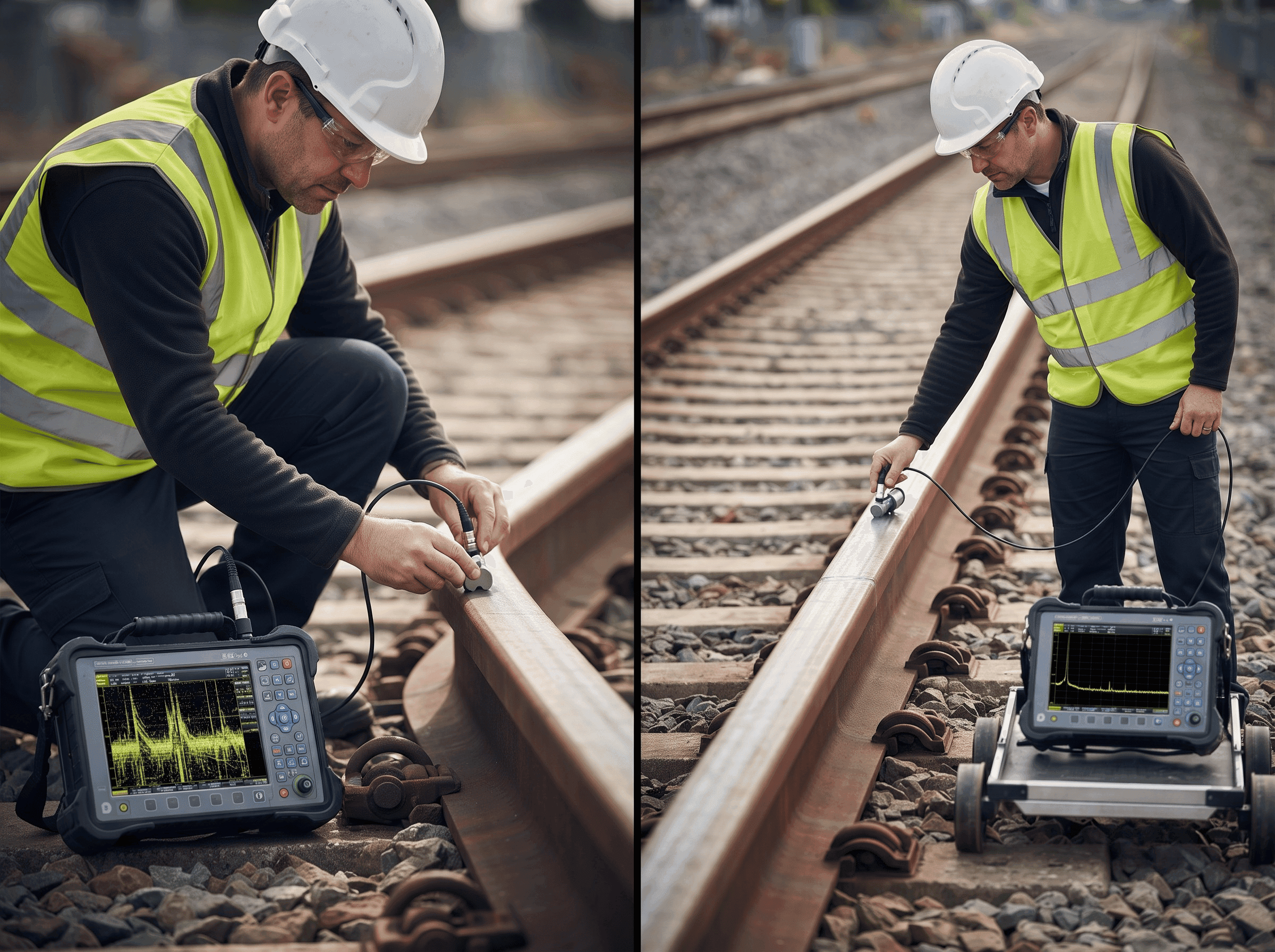
Near field vs far field in UT is the split between the zone in front of a probe where sound pressure swings through maxima and minima, and the zone beyond, where the beam spreads. The boundary is the near-field length, N = D²f/(4c). For a 0.5 in., 2.25 MHz probe in steel, N is about 15 mm (0.61 in.).
Inside N, echo amplitude is unreliable for sizing. Beyond N, amplitude falls in a predictable way with distance. This guide works the formula for straight-beam, angle-beam and rectangular probes, then shows what the numbers mean for thin sections, DAC curves, weld probes and rail probes. The underlying physics is covered briefly in EMA's pillar on the science behind ultrasonic testing; this article goes deeper into the calculations and the field decisions.
What is near field vs far field in UT?
The near field (Fresnel zone) is the region between the probe face and the last on-axis pressure maximum; the far field (Fraunhofer zone) is everything beyond it. In the near field, waves from different points on the element arrive at each spot with different path lengths, so they reinforce in some places and cancel in others. In the far field, those path differences become small and the beam behaves like a single expanding wave.
Evident's beam characteristics tutorial defines the zone this way and states the practical consequence:
"The near field is the region close to the transducer where the sound pressure goes through a series of maximums and minimums … it can be difficult to accurately evaluate flaws using amplitude based techniques." (Evident, Beam Characteristics)
The same tutorial notes that N is the transducer's natural focus and "represents the greatest distance at which a transducer's beam can be focused." A lens or phased-array delay law can pull the focus closer than N, never farther.
| Property | Near field (Fresnel zone) | Far field (Fraunhofer zone) |
|---|---|---|
| Where | Probe face to N | Beyond N |
| On-axis pressure | Rises and falls through maxima and minima | Falls steadily with distance |
| Beam width | Roughly the element width, with side structure | Spreads at a fixed half-angle |
| Echo amplitude vs reflector size | Unreliable | Predictable; the basis of DAC and DGS sizing |
| Depth (time-of-flight) readings | Valid | Valid |
| Main concern | Interference pattern | Beam spread and attenuation |
Key takeaway: the near field affects amplitude, not time of flight, so depth and thickness readings stay valid inside it.
How do you calculate near-field length?
For an unfocused circular element, N = D²/(4λ), and because λ = c/f, the same thing is N = D²f/(4c). D is the element diameter, f the center frequency, c the sound velocity of the wave mode in the material, and λ the wavelength. The Evident tutorial and the Waygate Technologies transducer catalog both give this form, the catalog adding that it holds when D is much larger than the wavelength.
| Symbol | Meaning | Unit used in this article |
|---|---|---|
| N | Near-field length, measured from the probe face along the beam axis | mm |
| D | Element diameter (or effective dimension; see below) | mm |
| f | Center frequency | MHz (cycles per µs) |
| c | Velocity of the wave mode in use | mm/µs |
| λ | Wavelength, c/f | mm |
A unit tip saves most arithmetic errors. With D in mm, f in MHz and c in mm/µs, the answer comes out in mm directly. Steel's longitudinal velocity of 5,890 m/s is 5.89 mm/µs, and its shear velocity of about 3,250 m/s is 3.25 mm/µs, both from the Evident material velocity table.
Three relationships follow from the formula:
- Diameter is squared. Doubling D quadruples N.
- Frequency is linear. Doubling f doubles N, because the wavelength halves.
- Velocity is inverse. The same probe has a longer near field in a slower material. In water (1.48 mm/µs) a probe's near field is about four times its near field in steel.
Key takeaway: always use the velocity of the wave mode that actually travels in the part: longitudinal for a 0° probe, shear for a normal angle-beam probe.
Worked example 1: 0° probes in steel
A 20 mm (0.79 in.), 5 MHz straight-beam probe has a near field of about 85 mm (3.34 in.) in steel. That is the figure the earlier version of this article referred to without showing the calculation. Here it is, with other common probes for comparison.
N = D² × f / (4 × 5.89), with 4 × 5.89 = 23.56.
| Element D | Frequency | λ in steel | Calculation | N in steel |
|---|---|---|---|---|
| 6.35 mm (0.25 in.) | 5 MHz | 1.18 mm | 40.32 × 5 / 23.56 | 8.6 mm (0.34 in.) |
| 10 mm (0.39 in.) | 2 MHz | 2.95 mm | 100 × 2 / 23.56 | 8.5 mm (0.33 in.) |
| 10 mm (0.39 in.) | 5 MHz | 1.18 mm | 100 × 5 / 23.56 | 21.2 mm (0.84 in.) |
| 12.7 mm (0.5 in.) | 2.25 MHz | 2.62 mm | 161.3 × 2.25 / 23.56 | 15.4 mm (0.61 in.) |
| 12.7 mm (0.5 in.) | 5 MHz | 1.18 mm | 161.3 × 5 / 23.56 | 34.2 mm (1.35 in.) |
| 20 mm (0.79 in.) | 2 MHz | 2.95 mm | 400 × 2 / 23.56 | 34.0 mm (1.34 in.) |
| 20 mm (0.79 in.) | 5 MHz | 1.18 mm | 400 × 5 / 23.56 | 84.9 mm (3.34 in.) |
| 25.4 mm (1.0 in.) | 1 MHz | 5.89 mm | 645.2 × 1 / 23.56 | 27.4 mm (1.08 in.) |
| 25.4 mm (1.0 in.) | 2.25 MHz | 2.62 mm | 645.2 × 2.25 / 23.56 | 61.6 mm (2.43 in.) |
| 25.4 mm (1.0 in.) | 5 MHz | 1.18 mm | 645.2 × 5 / 23.56 | 136.9 mm (5.39 in.) |
Check the 85 mm row the other way: λ = 5.89 / 5 = 1.178 mm, and N = 400 / (4 × 1.178) = 84.9 mm. Both forms agree.
Read the 85 mm figure as a zone boundary, not a cliff. The probe does not change behavior at exactly 85 mm. The last maximum is broad, and pulsed broadband probes smear the interference pattern, so treat roughly 0.5N to 1.5N as a transition region.
As a practical scale: 85 mm is close to half the 185.7 mm (7-5/16 in.) height of 136RE rail (supplier data, to be confirmed for the section in your track). A large, high-frequency 0° probe placed on the running surface would put the whole rail head and much of the web inside its near field.
Key takeaway: large-diameter, high-frequency probes push the near field deep; check N against the depth of the flaws you are looking for before choosing one.
How do you calculate the near field of an angle-beam probe?
For a shear-wave angle-beam probe, calculate N with the shear wavelength in steel, then subtract the part of the near field used up inside the wedge, and measure what remains along the sound path. Three corrections separate this from the 0° case: the wave mode, the wedge path and the direction of measurement.
- Use the shear wavelength. At normal wedge angles only a shear wave enters steel. At 2.25 MHz the shear wavelength is 3.25 / 2.25 = 1.44 mm, against 2.62 mm for the longitudinal wave. The shorter wavelength makes the near field longer by the ratio 5.89 / 3.25 = 1.81.
- Deduct the wedge path. Sound spends part of its near field in the plastic wedge. Convert the wedge path to a steel-equivalent distance by multiplying by c_wedge / c_steel(shear), then subtract it. The rule follows from scaling distance by wavelength in each medium.
- Measure along the sound path. The remaining N is a distance along the refracted beam, not a depth. Depth = sound path × cos(refracted angle).
Worked example 2: 70° probe on 1 in. plate
Inputs: a 5/8 × 5/8 in. (15.9 × 15.9 mm) square element, 2.25 MHz, 70° shear in steel (3.25 mm/µs), acrylic wedge (2.73 mm/µs, Evident table) with an assumed 15 mm acoustic path from element center to exit point. The wedge path is illustrative; take the real value from the probe data sheet. A square element uses Evident's aspect ratio constant k = 1.37 (explained in the next section).
| Step | Calculation | Result |
|---|---|---|
| Shear wavelength | 3.25 / 2.25 | 1.44 mm |
| Near field, total (shear) | 1.37 × 15.9² / (4 × 1.44) = 1.37 × 252.0 / 5.78 | 59.8 mm |
| Wedge path, steel-equivalent | 15 × 2.73 / 3.25 | 12.6 mm |
| Near field remaining in steel, along sound path | 59.8 − 12.6 | 47.2 mm (1.86 in.) |
| Depth where the near field ends | 47.2 × cos 70° = 47.2 × 0.342 | 16.1 mm (0.64 in.) |
| Surface distance at that point | 47.2 × sin 70° = 47.2 × 0.940 | 44.3 mm (1.75 in.) |
| First-leg sound path in 1 in. (25.4 mm) plate | 25.4 / 0.342 | 74.3 mm (2.92 in.) |
The near field ends about 64% of the way down the first leg, at a depth of about 16 mm in 25.4 mm plate. A reflector in the top 16 mm of the first leg sits in the near field. The second leg (74.3 to 148.5 mm sound path) is entirely in the far field.
Had the longitudinal velocity been used by mistake, the total would be 1.37 × 252.0 / (4 × 2.62) = 33.0 mm, and the error would hide most of the near field. The angle beam testing in UT article covers the probe index, angle check and skip geometry this example relies on.
Key takeaway: for angle-beam work, shear wavelength in, wedge path out, and the result is a sound-path distance.
How do you handle a rectangular element?
A rectangular or square element has no single diameter, so the formula needs an effective dimension. Evident's review of conventional beam characteristics multiplies the long dimension's square by an aspect ratio constant k that depends on the ratio of the short to the long side, giving N = k × L² × f / (4c). For circular elements, "k is not used and the diameter of the element (D) is used instead of the length term." The formula on that page is an image, so the expression here is our reading of it; confirm it before quoting.
| Short / long ratio | k (Evident) |
|---|---|
| 1.0 (square) | 1.37 |
| 0.9 | 1.25 |
| 0.8 | 1.15 |
| 0.7 | 1.09 |
| 0.6 | 1.04 |
| 0.5 | 1.01 |
| 0.4 | 1.00 |
| 0.3 and below | 0.99 |
A simpler method replaces the rectangle with a circle of equal area: D_eff = √(4ab/π). It usually lands within a few percent of the k method.
Worked example 3: checking both methods against a catalog
The Waygate catalog lists two Krautkrämer 70° probes with their near-field length in steel. Both are calculated here at 2 MHz, shear wavelength 3.25 / 2 = 1.625 mm, so 4λ = 6.5 mm.
| Probe (catalog) | Element a × b | Equal-area method | k method | Catalog N (steel) |
|---|---|---|---|---|
| WB 70-2 | 20 × 22 mm (0.79 × 0.87 in.) | D_eff² = 4 × 440 / π = 560.2; N = 560.2 / 6.5 = 86.2 mm | ratio 0.91, k ≈ 1.26; N = 1.26 × 22² / 6.5 = 93.9 mm | 90 mm (3.5 in.) |
| MWB 70-2 | 8 × 9 mm (0.31 × 0.35 in.) | D_eff² = 4 × 72 / π = 91.7; N = 91.7 / 6.5 = 14.1 mm | ratio 0.89, k ≈ 1.24; N = 1.24 × 9² / 6.5 = 15.4 mm | 15 mm (0.6 in.) |
Both methods land within about 5% of the published values, which bracket them. The k values for ratios 0.91 and 0.89 are interpolated from Evident's table. The catalog also lists the 4 MHz MWB at 30 mm, double the 2 MHz figure, as the formula predicts.
The catalog does not say whether its figure already deducts the wedge path. Probe data sheets are measured under EN ISO 22232-2:2020, the probe characterization standard that replaced EN 12668-2. Ask the manufacturer how its stated N is defined before deducting the wedge.
Key takeaway: for rectangles, use an effective dimension and cross-check the data sheet; two methods within 5% of each other are close enough to plan a scan.
Why is echo amplitude misleading inside the near field?
Inside the near field, the same reflector can give a larger or smaller echo at different depths, so amplitude no longer tracks reflector size. For an ideal continuous-wave piston, the on-axis pressure swings between zero and about twice its average value through the near field. Broadband pulsed probes smooth the swings, but they do not remove them.
Three consequences matter on the job:
- A small reflector near a pressure maximum can out-echo a larger one near a minimum. Ranking two near-field indications by amplitude can rank them wrongly.
- Moving the probe changes the echo even when the reflector does not change. The pressure pattern also varies across the beam, not just along it.
- Amplitude-based sizing assumes far-field behavior. DGS (AVG) diagrams are normally drawn with distance expressed in multiples of N, and their accuracy is weakest close to the probe. The Waygate catalog adds that "Focusing is only possible within the near field of the probe."
Time of flight is not affected. Evident notes that in the near field thickness gauging "is not a problem," because a thickness gauge reads the arrival time of the back-wall echo, not its height.
Key takeaway: in the near field, trust the depth reading and distrust the amplitude.
What does the near field mean in the field?
The near-field length should drive three decisions: which probe to use on thin sections, where the DAC or TCG reference points go, and which probe to choose for a given weld or rail section. Each is worked below.
Thin sections: delay-line and dual-element probes
A delay line or a dual-element probe moves the near field and the initial-pulse dead zone out of a thin part. Evident's thickness gauge transducer guide says a major reason for delay lines "is for thin material measurements," because the excitation pulse must be separated from the back-wall echoes. It describes duals as "used primarily for measurements involving rough, corroded surfaces," with two elements set at a small angle to focus at a chosen depth.
Worked numbers for a delay line on 6 mm (0.24 in.) steel, using a 6.35 mm, 5 MHz element and a 12.7 mm (0.5 in.) acrylic delay:
| Step | Calculation | Result |
|---|---|---|
| N in steel with no delay | 6.35² × 5 / (4 × 5.89) | 8.6 mm, deeper than the 6 mm part |
| Delay, steel-equivalent | 12.7 × 2.73 / 5.89 | 5.9 mm |
| Near field remaining in steel | 8.6 − 5.9 | 2.7 mm |
| Round trip in the delay | 2 × 12.7 / 2.73 | 9.30 µs |
| Round trip in 6 mm steel | 2 × 6 / 5.89 | 2.04 µs |
| Back-wall multiples before the delay repeat echo | 4 × 2.04 = 8.15 µs < 9.30 µs | 4 clean back-wall echoes |
Without the delay, the whole 6 mm part sits inside an 8.6 mm near field, and the first back-wall echo can be lost in the initial pulse. With it, most of the near field sits in the plastic, and four back-wall echoes arrive before the delay's own repeat echo.
A dual-element probe takes a different route. The transmitter and receiver are separate, so the receiver is not blinded by the initial pulse, and the roof angle crosses the beams at a shallow depth. Duals are the usual choice for corroded or pitted surfaces and shallow laminations. Their trade-off, per Evident, is that "measurement with duals is sometimes not as accurate as with other types of transducers," and sensitivity drops away from the beam crossing. EMA's dead zone in ultrasonic testing article covers the initial-pulse side of this problem, and thickness gauge or flaw detector covers instrument choice.
No DAC points in the near field
Good practice is to place DAC or TCG reference reflectors beyond the near field of the probe being used, unless the procedure says otherwise. A DAC curve joins the peak echoes from equal reflectors at several depths, and the instrument draws straight or smoothed lines between those points. In the far field that is sound, because the true response falls smoothly. In the near field, the response between two measured points can rise or dip, and the line drawn between them does not show it.
Evident's DAC and TVG tutorial says "A DAC curve graphically compensates for material attenuation, nearfield effects, and beam spreading." That is true at the depths actually measured. It does not make the curve reliable between points that sit in the near-field pattern.
Using worked example 2: the 5/8 in. 70° probe's near field ends at about 47 mm sound path. On an ASME-style 1 in. block at 70°, holes at 1/4 T and 1/2 T (6.35 and 12.7 mm deep) give first-leg sound paths of 6.35 / 0.342 = 18.6 mm and 12.7 / 0.342 = 37.1 mm, both inside the near field. The 3/4 T hole (19.05 mm deep) gives 55.7 mm, just beyond it. A smaller or lower-frequency probe, or second-leg reference points, may give a curve that is in the far field throughout; the procedure decides which is allowed.
| Hole (1 in. block, 70°) | Depth | First-leg sound path | Inside the 47 mm near field? |
|---|---|---|---|
| 1/4 T | 6.35 mm | 18.6 mm | Yes |
| 1/2 T | 12.7 mm | 37.1 mm | Yes |
| 3/4 T | 19.05 mm | 55.7 mm | No |
The DAC curve in ultrasonic testing article covers building and checking the curve itself.
Choosing a probe for a weld
For weld UT, choose the probe so the weld volume of interest is beyond, or mostly beyond, the near field along the sound path. Worked example 3 shows why size matters. On 1 in. (25.4 mm) plate at 70°, the first leg is 74.3 mm of sound path. With the WB 70-2's 90 mm near field, less an assumed 12.6 mm steel-equivalent wedge path, about 77 mm remains, so the entire first leg sits inside the near field. With the MWB 70-4 (8 × 9 mm, 4 MHz, 30 mm catalog), less an assumed 6.7 mm, the near field ends at about 23 mm of sound path, a depth of about 8 mm.
The code still governs the probe. Older editions of AWS D1.1, as quoted on the AWS forum, specify angle-beam crystals 5/8 to 1 in. wide and 5/8 to 13/16 in. high at about 2 to 2.5 MHz; confirm the exact limits in the edition named in your contract. D1.1 rates indications against a single side-drilled hole reference with a distance correction, while ASME Section V procedures build a DAC, so the near-field question shows up differently under each code. See AWS D1.1 weld inspection criteria for the rating method.
Choosing a probe for a rail head or web
On rail, the near field matters most for shallow head defects and for testing through the thin web. A horizontal split head is usually 1/4 in. (6.35 mm) or more below the running surface, under the definition in 49 CFR 213.113(d). A 0.5 in., 2.25 MHz 0° probe has a 15.4 mm near field, so a reflector at 6 to 15 mm lies inside it. A dual-element 0° probe or a delay probe gives a more dependable response there.
Testing through the web from the side is a thin-section job. The 136RE web is about 17.5 mm (11/16 in.) thick (supplier data, to be confirmed). A 1 in., 2.25 MHz probe's 61.6 mm near field would put the whole web inside it, while a 0.25 in., 5 MHz probe (8.6 mm) or a dual is a better match. Looking down from the running surface to the base, 185.7 mm away, most of the path is far field for common probes.
Rail search units on test cars are typically low-megahertz probes in fluid-filled wheels or sleds; one published patent (US 5,777,891) describes wheel transducers "typically centered at 2.25 Mhz." The fluid path holds part of the near field, which is one advantage of that design. Head checks and shelling can still mask what lies beneath them, whatever the probe. EMA's ultrasonic flaw detector for rail inspection article covers hand-test equipment.
Key takeaway: compute N for the probe you plan to use, compare it with the depth or sound path of the target, and change the probe before you change the interpretation.
How should inspectors evaluate an indication inside the near field?
An indication in the near field is still a real indication; what changes is how far its amplitude can be trusted. Work through these steps in order:
- Note the probe's element size, frequency, wave mode and wedge or delay path from the data sheet.
- Use the calibrated velocity for the part, not a table value, and compute N along the sound path.
- Compare the indication's sound path with N. If it lies inside about 1.5N, flag it as near-field.
- Re-examine with a probe that puts the indication in the far field: a smaller or lower-frequency element, a dual, a delay line, or a different angle or leg.
- Where possible, size by a method that does not depend on absolute amplitude, such as probe-movement (6 dB drop) length sizing or tip diffraction, as the procedure allows.
- Record the probe, the near-field length and the method used, then apply the procedure's acceptance criteria.
The procedure remains the authority. Near-field position is a reason to re-examine, not a reason to accept or reject an indication automatically. The ultrasonic testing formulas article collects the depth and beam-spread formulas used alongside these steps.
What are the limits of the near-field formula?
N = D²f/(4c) is an approximation for an ideal, unfocused, continuous-wave piston source, and real probes depart from it. Use it to plan; use the data sheet and a beam check to confirm.
| Limit | What it means in practice |
|---|---|
| Assumes D much larger than λ | Very small elements at low frequency follow the formula poorly |
| Assumes an unfocused, flat element | Lensed and phased-array probes have a focal distance shorter than N; use the manufacturer's beam data |
| Broadband pulses | The pattern is smoothed and the last maximum is broad, so N is a zone, not a line |
| Nominal vs actual frequency | A probe marked 5 MHz may measure differently; N moves in proportion |
| Velocity | Table velocities are "only a general guide" (Evident); calibrate on the part |
| Rectangular and wedge corrections | Effective dimensions and wedge deductions are approximations; probe data sheets are measured under EN ISO 22232-2 |
| Curved and rough surfaces | Contact geometry changes the effective aperture and the beam |
| Coarse grain and anisotropic welds | Scattering and beam skewing in austenitic welds or cast manganese distort the field beyond what the formula describes |
The formula also says nothing about the dead zone, which is the initial-pulse ring-down at the surface. A probe can have a short near field and still miss a reflector 1 mm deep.
How EMA Industries applies this
EMA Industries is a Southern California NDT contractor that mobilizes nationwide. It provides ultrasonic rail flaw testing for transit agencies, short lines and industrial track owners, rail weld inspection, AWS D1.1 structural weld UT, and NDT Level III services, including written UT procedures and probe selection. Near-field checks of this kind belong in a procedure's probe and calibration sections. To discuss a weld or rail inspection, see ultrasonic examination or contact EMA Industries.
Frequently asked questions
How do you calculate the far-field distance?
The far field starts at the near-field length, N = D²f/(4c), or D²/(4λ). For a 1 in., 2.25 MHz probe in steel, N = 25.4² × 2.25 / (4 × 5.89) = 61.6 mm (2.43 in.). Beyond that point the on-axis pressure falls steadily, and amplitude comparisons become dependable.
What is meant by the near field in ultrasonic testing?
The near field is the region in front of the probe, from the face to distance N, where waves from different parts of the element interfere. The sound pressure rises and falls through a series of maxima and minima, so echo amplitude does not track reflector size reliably. It is also called the Fresnel zone.
Does the near field affect thickness measurement?
Thickness readings use time of flight, not amplitude, so the near field does not invalidate them. Evident states that thickness gauging in the near field "is not a problem." The practical limit on very thin parts is the initial pulse, which is why delay-line and dual-element probes are used on thin sections.
Why does a higher frequency give a longer near field?
A higher frequency has a shorter wavelength, and N = D²/(4λ), so N grows in direct proportion to frequency. A 0.5 in. probe in steel has a near field of 15.4 mm at 2.25 MHz and 34.2 mm at 5 MHz. Higher frequency improves resolution but pushes the zone of unreliable amplitude deeper.
Is the near field of an angle-beam probe the same as a straight-beam probe?
The two differ for three reasons. The angle-beam calculation uses the shear wavelength, which makes N about 1.8 times longer in steel than the longitudinal value for the same element. Part of the near field lies in the wedge and is deducted. The remainder is measured along the refracted sound path, so its depth is the sound path times the cosine of the angle.
Sources
- Evident, Beam Characteristics (near-field definition, formula, focusing limit, thickness gauging): https://ims.evidentscientific.com/en/learn/ndt-tutorials/flaw-detection/beam-characteristics
- Evident, A Review of Conventional Beam Characteristics (aspect ratio constant k for rectangular elements): https://ims.evidentscientific.com/en/learn/ndt-tutorials/transducers/characteristics
- Evident, Material Sound Velocities (steel, acrylic, water): https://ims.evidentscientific.com/en/learn/ndt-tutorials/thickness-gauge/appendices-velocities
- Evident, Transducer Types (delay-line and dual-element probes): https://ims.evidentscientific.com/en/learn/ndt-tutorials/thickness-gauge/transducers
- Evident, DAC and TVG: https://ims.evidentscientific.com/en/learn/ndt-tutorials/flaw-detection/dac-tvg
- Waygate Technologies (Krautkrämer), Ultrasonic Transducers catalog, near-field definition and WB/MWB angle-probe data (manufacturer document): https://core.instrumart.com/assets/waygate-transducer-catalog.pdf
- EN ISO 22232-2:2020, Non-destructive testing — Characterization and verification of ultrasonic test equipment — Part 2: Probes (SIS catalog listing): https://www.sis.se/produkter/provning-4361e6b5/oforstorande-provning/ss-en-iso-22232-22020/
- 49 CFR 213.113, Defective rails (horizontal split head definition), eCFR: https://www.ecfr.gov/current/title-49/subtitle-B/chapter-II/part-213/subpart-D/section-213.113