Ultrasonic testing (UT) is a nondestructive testing method that sends high-frequency sound, usually 1 to 10 MHz, into a part and times the echoes that come back from flaws and back walls. In steel a longitudinal wave travels about 5,890 m/s, so every microsecond of round-trip time equals roughly 0.116 in. of depth.
That single relationship, time multiplied by velocity, is what lets an inspector say not just "there is something inside this weld" but "there is a reflector 1.39 in. below the surface, 2 in. from the toe". The rest of UT practice is about choosing the right wave, angle and frequency so the flaw you care about actually sends sound back to the probe.
This page is the entry point to EMA Industries' UT library. It explains the principle with real numbers, gives one line on each technique with a link to the deeper article, sets out what UT finds and misses, and names the codes and rules that govern it, including internal rail flaw testing under 49 CFR 213.237.
What is ultrasonic testing?
Ultrasonic testing is a volumetric NDT method: it looks inside a part with sound above the range of human hearing and reports where the sound was reflected. It doesn't damage the part, it needs access from only one side for most techniques, and it gives a depth reading directly from the time base.
Human hearing tops out at about 20 kHz. Industrial flaw detection works far above that. Evident's flaw detection tutorial puts it this way: "the majority of ultrasonic flaw detection applications utilize frequencies between 500,000 and 10,000,000 cycles per second." Contact weld and rail work in steel mostly sits between 1 and 5 MHz, with 2.25 MHz the long-standing choice for rail test wheels.
UT is used on welds, plate, forgings, castings, pipe, bolts and rail. It is one of the two volumetric NDT methods, alongside radiography (RT). Surface methods such as magnetic particle (MT) and penetrant (PT) complement it rather than compete with it.
Industrial ultrasonic testing is not medical ultrasound. The physics is related, but the equipment, frequencies, codes and qualifications are entirely separate, and nothing on this page applies to diagnostic imaging.
Key takeaway: UT locates internal reflectors by timing sound in a material whose velocity is known.
How does ultrasonic testing work?
A UT instrument fires a short electrical pulse into a piezoelectric transducer, the transducer turns it into a sound pulse, and the same or a second transducer turns returning echoes back into a voltage that is plotted against time. That plot is the A-scan: amplitude on the vertical axis, time (and so sound path) on the horizontal axis.
The chain has five parts:
- Pulser-receiver. It excites the transducer and amplifies the weak returning signal. Gain is set in decibels; a 6 dB change halves or doubles the echo amplitude.
- Transducer (probe). A piezoelectric element, from about 0.25 in. to 1 in. across for contact work, sets the frequency and beam size.
- Wedge or delay line. A plastic wedge refracts the beam to an angle such as 45°, 60° or 70°. A delay line puts a known stand-off between the element and the part.
- Couplant. Gel, oil, glycerin-water mix or water fills the gap between probe and part. Steel against air reflects almost all of the sound, which is why a dry probe shows nothing.
- Display and time base. The instrument is calibrated on a reference block so that a given time equals a known distance in the material being tested.
The physics behind each step, including Snell's law, mode conversion, near field and beam spread, is covered in depth in the science behind ultrasonic testing. The essentials are below.
Velocity, frequency and wavelength
Sound velocity is a property of the material and the wave type, and wavelength follows from it: λ = v ÷ f. Longitudinal (compression) waves are used for straight-beam testing; shear waves, which travel at a little over half the speed, are used for most angle-beam weld and rail testing.
| Material and wave | Velocity | Velocity (in./µs) | Wavelength at 1 MHz | at 2.25 MHz | at 5 MHz | at 10 MHz |
|---|---|---|---|---|---|---|
| Steel, longitudinal | 5,890 m/s | 0.232 | 5.89 mm | 2.62 mm | 1.18 mm | 0.59 mm |
| Steel, shear | 3,250 m/s | 0.128 | 3.25 mm | 1.44 mm | 0.65 mm | 0.33 mm |
| Water (immersion and wheel probes) | 1,480 m/s | 0.058 | 1.48 mm | 0.66 mm | 0.30 mm | 0.15 mm |
Longitudinal steel and water velocities: Evident material sound velocity table (1020 steel). Shear: Evident steel wedge design value. Wavelengths calculated. Treat every figure as a starting point: Evident notes its velocities are "only a general guide", and real steels differ by about 1%, which is why the instrument is calibrated on the same material.
Why frequency matters
Higher frequency gives a shorter wavelength, better resolution and sensitivity to smaller reflectors; lower frequency penetrates further through coarse grain and heavy sections. A common training rule of thumb is that a reflector about half a wavelength across is near the limit of reliable detection, so 5 MHz in steel (λ/2 ≈ 0.6 mm longitudinal) sees smaller features than 1 MHz (λ/2 ≈ 2.9 mm). It is a rule of thumb, not a code requirement; orientation and surface condition matter as much as size.
The trade-off is attenuation. Grain scattering rises steeply with frequency, so castings, austenitic stainless welds and very thick sections are tested at 0.5 to 2.25 MHz, while thin plate, thickness gauging and near-surface work use 5 to 10 MHz or more.
From echo time to position
For a straight (0°) beam, depth = v × t ÷ 2, because the sound goes down and back. For an angle beam, the instrument divides the round trip the same way to get the sound path, then resolves it: depth = sound path × cos θ and surface distance = sound path × sin θ, where θ is the refracted angle. If the sound path is longer than one leg (thickness ÷ cos θ), the beam has bounced off the back wall and the depth must be worked out on the second leg.
Worked example: depth from time of flight
These three cases use the velocities in the table above and assume the instrument zero (wedge and delay time) has already been subtracted, as it is after calibration.
Case 1: straight beam in 2.00 in. steel plate
| Step | Calculation | Result |
|---|---|---|
| Velocity | Steel, longitudinal | 0.232 in./µs |
| Expected back-wall echo | 2 × 2.00 ÷ 0.232 | 17.24 µs |
| Indication | Echo at 12.0 µs | — |
| Depth | 0.232 × 12.0 ÷ 2 | 1.392 in. |
| Check | 1.392 < 2.00 in. plate | Inside the plate |
An echo at 12.0 µs, ahead of the 17.24 µs back wall, is a reflector about 1.39 in. deep. A lamination at that depth would usually also reduce the back-wall echo.
Case 2: 45° shear wave in 1.00 in. plate (second leg)
| Step | Calculation | Result |
|---|---|---|
| Velocity | Steel, shear | 0.128 in./µs |
| Indication | Echo at 30.0 µs | — |
| Sound path | 0.128 × 30.0 ÷ 2 | 1.920 in. |
| End of first leg | 1.00 ÷ cos 45° | 1.414 in. |
| Leg | 1.920 > 1.414 | Second leg |
| Depth | 2 × 1.00 − 1.920 × cos 45° = 2.00 − 1.358 | 0.642 in. |
| Surface distance from probe exit point | 1.920 × sin 45° | 1.358 in. |
The tempting answer, 1.920 × cos 45° = 1.358 in., is deeper than the 1.00 in. plate, which is impossible. The beam has reflected off the back wall, so the reflector is 0.642 in. below the scanning surface. Checking depth against thickness on every angle-beam call catches this error.
Case 3: 70° shear wave in a rail head
| Step | Calculation | Result |
|---|---|---|
| Indication | Echo at 37.5 µs | — |
| Sound path | 0.128 × 37.5 ÷ 2 | 2.40 in. |
| Depth below the running surface | 2.40 × cos 70° | 0.821 in. |
| Distance ahead of the probe | 2.40 × sin 70° | 2.255 in. |
A reflector 0.82 in. down is within the head of a typical heavy rail section, where transverse defects grow. One microsecond of error at 70° moves the depth only about 0.022 in. but the position along the rail about 0.060 in., which is why hand verification of a test-car indication relies on careful marking. More time-of-flight checks are collected in ultrasonic testing formulas.
What are the steps of the ultrasonic testing process?
A contact ultrasonic testing process runs in seven steps: prepare the surface, choose the probe, calibrate distance and sensitivity on reference blocks, plan the scan, scan with couplant, evaluate each indication against the acceptance criteria the contract names, and record the result. The order matters. The probe is chosen before calibration because the instrument is calibrated with that probe, and the acceptance criteria are fixed before scanning because they set the level at which an echo must be recorded.
The steps below describe manual pulse-echo testing of welds and plate. A rail test car follows the same logic, with calibration on a reference rail and the scan plan built into the probe wheel, as described in how rail UT is done.
| Step | What is done | What goes wrong when it is skipped |
|---|---|---|
| 1. Surface preparation | Remove spatter, loose scale, loose paint, dirt and grease from the scanning surface on both sides of the weld | Lost coupling; a stretch with no coupling is untested, not sound |
| 2. Probe selection | Choose frequency, element size and refracted angle for the flaw sought and the section thickness | The wrong angle misses the bevel face; the wrong frequency scatters in coarse grain |
| 3. Calibration | Set velocity and zero on a reference block, then the reference sensitivity on a specified reflector; build a DAC or TCG curve if the procedure uses one | Depth and position read wrong; echo heights can't be compared with the acceptance level |
| 4. Scan plan | Fix the surfaces, sides, angles, index step and scanning gain | Part of the weld volume is never insonified |
| 5. Scanning | Move the probe in the planned pattern with couplant, watching the A-scan | Gaps between passes; second-leg coverage missed |
| 6. Evaluation | Maximize each indication, read its level and sound path, locate it and rate it against the acceptance criteria | Reflectors accepted or rejected on echo height alone |
| 7. Recording | Record the instrument, probe, block, settings, couplant, scan and every reportable indication, then sign | The test can't be repeated or audited |
Step 1: surface preparation
Contact UT needs a surface the probe can couple to. Procedures commonly require removal of weld spatter, loose scale and loose paint from the scanning surface, which for an angle-beam weld test is the base metal on both sides of the weld out to the full skip distance. Tight mill scale and well-bonded paint are often allowed to stay if the procedure says so, usually with a check that the coating doesn't change the calibrated response. "Grind to bare metal" is more than most procedures ask, and it can leave a rougher surface than the one it replaced.
Step 2: probe selection
Frequency is a probe choice, not an instrument setting. The technician picks a probe, and with it a nominal frequency, element size and wedge angle, for the material and the flaw being sought; the instrument is then calibrated with that probe. Steel welds are mostly tested at 2.25 to 5 MHz, and coarse-grained material at 0.5 to 2.25 MHz, for the reasons given under why frequency matters. For angle-beam weld testing the refracted angle is chosen so the beam meets the bevel face near-normal; AWS D1.1-based procedures hold the angle within about 2° of 70°, 60° or 45° and assign angles by weld thickness and zone, so check the edition the contract names. A 0° straight-beam scan of the base metal beside the weld usually comes first, to find laminations that would block the angle beam.
Step 3: calibration on reference blocks
Evident's calibration tutorial separates three things that are all called "calibration". The first is velocity and zero calibration, "which must be performed whenever a new test material or transducer is being used". The second is reference calibration, "establishing a signal amplitude level from a reference standard for comparison to indications from the test piece". The third is periodic certification of the instrument itself. The same tutorial notes: "In flaw detection applications, two point calibration is frequently performed with an IIW reference block."
| Block | Size and features | What it is used for |
|---|---|---|
| IIW Type 1 (ISO 2400; ASTM E164 IIW-type) | 300 × 100 × 25 mm (12 × 4 × 1 in.) mild steel, 100 mm (4 in.) radius, 1.5 mm (0.060 in.) side-drilled hole, 50 mm hole | Time base (two-point velocity and zero), probe index and angle checks, and the reference level in AWS D1.1 work |
| IIW Type 2, V2 (ISO 7963) | About 75 × 43 × 12.5 mm, 25 and 50 mm radii, 5 mm hole | Field checks of miniature shear-wave probes: index, angle, time base and gain |
| Distance-amplitude block (ASME-style basic calibration block) | Side-drilled holes at 1/4, 1/2 and 3/4 of the thickness, in material like the part | Building a DAC or TCG curve |
The Type 1 block has no flat-bottom holes and no ladder of holes at different depths, so a DAC curve needs a separate distance-amplitude block. Evident's DAC tutorial: "Both DAC curves and TVG are commonly set up using a series of reference reflectors", one reflector size at several depths; the time-varied gain version raises the gain with sound path "to bring all of the reference echoes to the same height, typically 80%". An echo from a reflector the same size as the calibration reflectors then matches the curve at any depth; bigger reflectors plot above it, smaller below. The curve, and where its evaluation and recording levels sit, is explained in DAC curves in ultrasonic testing.
The reference level is set on the reflector the code names. AWS D1.1 sets it on the 0.060 in. side-drilled hole of the IIW-type block, and that single level, not a DAC curve, is the "b" in its indication rating. ASME Section V, Article 4 work uses the DAC from the basic calibration block instead. Which one applies is a contract question, not a technician's choice.
How often to recalibrate is set by the procedure, not by a standard. ASTM E317-21, the practice for evaluating instrument performance, says in clause 5.7 that no frequency of evaluation is "recommended or implied". D1.1-based procedures are reported to recheck calibration at least every 30 minutes and whenever the operator changes or power is interrupted; confirm the figure in the edition your contract names. For hand-held rail testing there is less structure: FRA report ORD-26/07 (ENSCO, July 2026) found no standardized calibration procedure among North American railroads, with zero, velocity, angle and gain typically set to 80% screen height on a known flaw, usually with an IIW Type 2 block, and it reported that no two operators in its trial produced statistically similar calibration results.
"Calibration errors can cause excessive false positives and false negatives." — FRA, DOT/FRA/ORD-26/07, Application of MAPOD to Handheld Ultrasonic Rail Flaw Inspection (2026)
What a rail owner should ask a contractor to show about calibration is set out in ultrasonic testing calibration for rail inspection RFPs.
Step 4: scan plan
A scan plan says which surfaces, which sides of the weld, which angles and what index step will be used, so that the whole weld volume is covered on at least one leg. D1.1-based procedures test from both sides of the weld axis wherever mechanically possible; a second angle is added where the bevel geometry or thickness calls for it. The index step between passes is the point most often skipped in generic descriptions. Evident's common test pattern moves the probe to and from the weld and "at each pass it is indexed by approximately one-half its width"; procedures based on ASME Section V, Article 4 set a minimum overlap of 10% of the transducer dimension perpendicular to the scan direction and a maximum scan speed of about 6 in./s unless calibration is verified at speed. Those ASME-based procedures also scan at a gain of at least twice the primary reference level (6 dB above it) and evaluate at the reference level, so that weak reflectors are not missed during the search.
Step 5: scanning with couplant
Couplant is there to remove the air film, not to "match" steel. Steel against air reflects almost all the sound, which is why a dry probe shows nothing; even a perfect water film still reflects most of the energy at the steel surface, and a thin film transmits enough. Use the same couplant for calibration and scanning, as ASME-based procedures require, because a change in couplant changes the transfer loss. The probe is moved in the planned raster, with a few degrees of swivel at each pass; Evident's tutorial notes that "the angulation helps in detection of inclusions, porosity, and other irregularly shaped reflectors". A separate pass along the weld, with the beam pointing along the axis, looks for transverse cracks. Throughout, the operator watches the A-scan for the signs of lost coupling, and any stretch scanned without coupling is recorded as untested rather than clear. Couplant choice for cold, grease and contaminated rail is covered in ultrasonic couplant for rail inspection.
Step 6: evaluation against the acceptance criteria
The technique standard tells the inspector how to look; the acceptance criteria tell the inspector what to do with what is found, and they come from a different document. ASTM E164-24, the practice for contact UT of weldments, puts the responsibility where it belongs: "there should be agreement between the manufacturer and the purchaser as to the specific reference standards", and "A detailed procedure for weld examination describing allowable discontinuity limits should be written and agreed upon."
Each indication is maximized, its sound path converted to depth and surface distance as in the worked example, its length taken by probe movement, and its level compared with the code's reference. Under AWS D1.1 that comparison is the indication rating d = a − b − c, where a is the indication level in dB, b the reference level from the 0.060 in. hole, and c the attenuation factor, 2 dB for every inch of sound path beyond the first.
Worked rating. An indication is brought to reference height at a = 38 dB. The reference hole needed b = 30 dB. The sound path is 3.5 in., so c = 2 × (3.5 − 1) = 5 dB, and d = 38 − 30 − 5 = +3 dB. Whether +3 dB is Class A (rejectable at any length), B, C or D depends on the weld thickness, the probe angle and whether the structure is statically or cyclically loaded, which is why the number alone decides nothing. A lower (more negative) d is a stronger reflector, so Class A sits at the low end of the table. The static-versus-cyclic qualifier and the class tables are worked through in AWS D1.1 weld inspection criteria.
Under ASME-based procedures the comparison is with the DAC curve: indications above the recording level are sized and compared with the referencing code's limits. On rail, each test-car indication is verified by hand before it becomes a defect under 49 CFR 213.113, which then sets the remedial action.
Step 7: recording
A UT report must let someone repeat the test. Procedures based on ASME Section V, Article 4 require the record to list the instrument, the search unit (frequency, size and angle), the calibration block and reference reflector, the reference level and scanning gain, the couplant (brand name or type), the surface condition, the surfaces and sides scanned, each reportable indication with its level, sound path, depth, surface distance, length and location, the disposition, and the examiner's name, certification level and date. D1.1 reports carry the same information plus the indication rating and class. For rail flaw testing, the records required by 49 CFR 213.241 sit on top of the contractor's own test and calibration records.
Key takeaway: write the ultrasonic testing process down as a procedure before the first scan, because the instrument only reports what the setup let it see.
What are the main ultrasonic testing techniques?
There are many UT techniques, not two. Most are variants of pulse-echo, where one probe (or one probe housing) both sends and receives. They differ in beam angle, how the probe is coupled, how many elements fire, and what signal is used for sizing.
| Technique | One-line description | Typical use | Read more |
|---|---|---|---|
| Pulse-echo, straight beam (0°) | Longitudinal wave normal to the surface; times echoes from reflectors parallel to the surface and the back wall | Laminations in plate, horizontal rail head splits, loss of back wall | Pulse-echo ultrasonic inspection |
| Pulse-echo, angle beam | Wedge refracts a shear wave to 45°, 60° or 70° to hit planar flaws that stand across the beam | Groove welds, transverse defects in rail heads | Angle beam testing in UT |
| Through-transmission | Separate transmitter and receiver on opposite sides; a flaw shows as a drop in received signal | Composites, bonded panels, some plate and bar lines; gives no depth | Types of ultrasonic testing in NDT |
| Immersion | Part and probe under water; the water path couples the sound and allows focusing and automated scanning | Shop inspection of bar, tube, forgings, aerospace parts (ASTM E1001) | Types of ultrasonic testing in NDT |
| Phased array (PAUT) | A multi-element probe steers and focuses the beam electronically, sweeping many angles and building an image | Weld inspection with encoded records (ASTM E2700) | UT vs PAUT |
| Time of flight diffraction (TOFD) | Two angled probes in pitch-catch time the weak signals diffracted from crack tips to measure through-wall height | Height sizing in welds, paired with pulse-echo or PAUT (ASTM E2373) | Types of ultrasonic testing in NDT |
| Thickness gauging | 0° pulse-echo reading of remaining wall from the back-wall time | Corrosion and erosion surveys (ASTM E797) | Ultrasonic thickness gauge |
| Guided wave (long-range UT) | Low-kHz waves that travel along a pipe or rail from one point, screening many feet for wall loss | Pipe screening; rail research and break detection (ASTM E2775) | Guided wave ultrasonic testing |
Three points keep this table honest:
- PAUT is pulse-echo. It changes how the beam is formed and displayed, not the underlying principle. It still needs calibration, a qualified operator and, for sizing, caution: ASTM E2700 warns that "extreme caution should be used when attempting to size indications using phased array".
- TOFD doesn't use the pulse-echo depth formula. It calculates depth from the diffraction geometry between two probes, and it has dead zones near the scanning surface and the back wall, so it is normally combined with pulse-echo or PAUT.
- Guided wave and long-range UT are the same method under two names. ASTM E2775 describes guided wave testing as "previously known as long range ultrasonic testing (LRUT)".
The pros and cons of each family, set side by side, are in advantages and disadvantages of ultrasonic testing.
How well does pulse-echo see flaws near the surface?
Pulse-echo is strongest at depth; close to the scanning surface its performance depends on the probe design and how the instrument is gated. It is not "especially good for surface and near-surface defects", and it is not blind near the surface either. The accurate answer sits between those two claims.
Where the near-surface limit comes from
With a single-element contact probe, the element is still ringing from the transmit pulse when the earliest echoes return. That ring-down, plus the interface signal, hides a short zone just under the surface, often called the dead zone. Its depth depends on frequency, damping and the instrument, so it is measured on a block rather than assumed. The dead zone article shows how.
The near field adds a second effect. Close to a 0° probe the beam has pressure peaks and nulls, so echo amplitude there is unreliable for sizing. For a 0.5 in., 2.25 MHz probe in steel the near field runs to about 0.61 in. (near field vs far field).
How practice overcomes it
- Dual-element probes separate transmit and receive elements, so the receiver isn't swamped by the transmit pulse. They are the normal choice for thin wall and corrosion work.
- Delay lines move the transmit pulse and interface echo off the part. Evident describes their use "where it is important to separate the excitation pulse recovery from back wall echoes."
- Angle beams reach near-surface material along a longer path. At 70°, every inch of depth is 2.92 in. of sound path, so a reflector just under the surface sits well clear of the initial pulse on screen.
- Water paths in immersion tanks and fluid-filled rail wheels do the same job as a delay line.
Gating and resolution
A gate is a time window on the A-scan that the instrument or test car monitors for echoes above a set threshold. Gates start after the interface or surface noise, so material shallower than the gate start is not evaluated by that channel. On rail, the practical near-surface limits are surface noise that must be gated out and scattering from rolling contact fatigue and shelling, not a general blind zone.
Resolution is the ability to show two close reflectors as two echoes. It improves with higher frequency and a shorter, better damped pulse. Near-surface resolution is a probe property you select for, which is why the procedure names the probe.
Key takeaway: choose a dual, delay-line or angle-beam setup for near-surface work, and verify the gate start on a reference block.
What does ultrasonic testing find?
UT is best at planar flaws, such as cracks and lack of fusion, that present a face to the beam, and at measuring depth and remaining thickness. It also finds volumetric flaws, though RT usually images those more clearly.
| Flaw or measurement | UT performance | Why |
|---|---|---|
| Cracks across the beam | Strong | A planar face reflects most of the sound back |
| Lack of sidewall fusion | Strong with the right angle | The bevel face must be near-normal to the beam; the angle is chosen for the bevel |
| Laminations in plate | Strong with 0° | Parallel to the surface, face-on to a straight beam |
| Through-wall height | Good with tip diffraction or TOFD | Time-based, not amplitude-based |
| Remaining wall thickness | Very good | Back-wall time with calibrated velocity |
| Slag and porosity | Fair | Rounded reflectors scatter sound in many directions |
| Cracks parallel to the beam | Poor | Edge-on to the beam, little energy returns |
| Flaw type identification | Indirect | Inferred from echo shape, position and probe angle |
An A-scan doesn't show a flaw's shape. Position comes from the sound path, length from scanning the probe along the indication, and type from the operator's judgment against weld geometry.
What are the limits of ultrasonic testing?
UT can only report what sends sound back to the probe, through material the sound can cross, examined by a person qualified to read it. Each limit below is a reason a procedure, not just an instrument, is needed.
| Limit | Effect | What is done about it |
|---|---|---|
| Orientation | A flaw parallel to the beam returns little energy | Scan with more than one angle and from both sides |
| Coarse grain | Austenitic welds, cast manganese frogs and some castings scatter and bend the beam | Lower frequency, refracted longitudinal probes, or another method |
| Surface condition | Rough, painted or scaled surfaces cut coupling; paint read at steel velocity distorts thickness | Surface preparation, coating correction, dual probes |
| Geometry | Thin sections, small diameters and complex shapes create confusing echoes | Contoured wedges, mockups, PAUT or RT |
| Near-surface zone | Single-element contact probes don't evaluate the first fraction of an inch | Duals, delay lines, angle paths, plus MT or PT for surface-breaking flaws |
| Masking | A shell or surface defect on rail can block sound from a flaw beneath it | Note the location as a possible untested area; follow-up testing |
| Sizing | Amplitude depends on orientation and roughness, so echo height alone doesn't give size | Length by probe movement; height by tip diffraction or TOFD |
| Operator dependence | Interpretation needs training and experience | Written procedures and certified personnel |
None of these limits are reasons to avoid UT. They are the reasons a contract specifies the technique, the reference standard and the acceptance criteria, and why a quiet screen with lost coupling must be recorded as untested, not as sound material.
Which codes and qualifications govern UT?
UT has three layers of documents: who may do it, how it is done, and what is accepted. Mixing them up is one of the most common errors in UT writing.
| Document | What it covers | What it doesn't do |
|---|---|---|
| ASNT SNT-TC-1A (2024) | A recommended practice for the employer's written practice: training hours, experience, exams and Levels I, II and III | ASNT doesn't certify anyone under it; the employer certifies |
| ANSI/ASNT CP-189 (2024) | A standard setting minimum requirements for employer-based certification | Still employer certification |
| ASME BPVC Section V, Article 4 | Ultrasonic examination methods for welds, including PAUT appendices, when invoked by a referencing code | Sets no acceptance criteria; those come from Section VIII, B31.3 or the referencing code |
| AWS D1.1, Clause 8 Part F | UT of groove welds in structural steel, about 5/16 to 8 in. thick, rated by the indication rating d = a − b − c | Doesn't by itself require UT; the contract or AISC does |
| 49 CFR 213.237 | Internal rail inspection intervals, valid search and joint-bar capability for Class 3–5 track | Names no test method |
| 49 CFR 213.238 | Qualified operators of rail flaw detection equipment: documented training, at least 160 h supervised experience, written authorization | Has no Level I/II/III structure; FRA doesn't certify operators |
Technique standards from ASTM, such as E164 for contact weld UT and E2700 for PAUT, describe how to examine; the purchaser or code names the acceptance level. D1.1 clause and table numbers changed in the 2020 reorganization (inspection moved to Clause 8), so check the edition named in the contract.
More detail: SNT-TC-1A requirements, AWS D1.1 weld inspection criteria, ASME weld ultrasonic inspection and UT acceptance criteria standards.
Key takeaway: a UT report should name the certification basis, the technique standard and the acceptance criteria separately.
How is ultrasonic testing used to inspect rail?
In the United States, internal rail flaw testing on Class 3, 4 and 5 track is required by 49 CFR 213.237, and the industry meets that requirement with ultrasonic testing. The rule itself requires the inspection, not the method. Paragraph (a) opens: "In addition to the inspections required by § 213.233, each track owner shall conduct internal rail inspections".
What the rule requires
- Interval. On Class 4 and 5 track, and on Class 3 track with scheduled passenger trains or a hazardous materials route, tests can be no more than 370 days or 30 million gross tons apart, whichever comes first. Other Class 3 track follows a longer schedule with a 5-year cap. Class 6 and higher falls under 213.339.
- Valid search. Section 213.237(j)(4) defines it (quoted in full below). Where a valid search couldn't be made, the owner must, before the interval runs out, make a valid search, cut speed to no more than 25 mph until one is made, or replace the rail.
- Joint bars. Under 213.237(f), "Inspection equipment shall be capable of detecting defects between joint bars, in the area enclosed by joint bars."
- Operators. Under 213.238, the provider must train, qualify and authorize each operator for the specific equipment type.
"Valid search means a continuous inspection for internal rail defects where the equipment performs as intended and equipment responses are interpreted by a qualified operator as defined in § 213.238." — 49 CFR 213.237(j)(4)
The definition matters for UT practice: a stretch where the probes lost coupling is not a valid search, even if the screen showed no defect.
The full rule, with worked tonnage examples, is in 49 CFR 213.237 rail flaw detection requirements and how often must rail be tested.
How rail UT is done
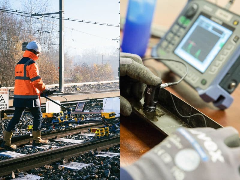
Rail can only be reached from the running surface, so in-track flaw detection is pulse-echo; through-transmission isn't used in track. Test cars, hi-rail units and walking carts carry probes in fluid-filled wheels or sleds that roll on the head, with water spray as couplant. One patent describes wheel-probe transducers "typically centered at 2.25 Mhz".
A typical probe set is:
- 70° shear for transverse defects in the head, such as transverse fissures and detail fractures
- 0° longitudinal for horizontal splits and loss of the base echo, which flags vertical splits, piped rail and other defects the beam can't see directly
- about 37–45° for bolt-hole cracks and web defects, plus side-looking probes on some systems
Each indication from a moving test is verified by hand before it is reported as a defect under 49 CFR 213.113, which then sets the remedial action.
Detection is good but not complete. TTCI (now MxV Rail) research describes conventional rail UT as finding "about 90 percent" of flaws during periodic inspection (Technology Digest TD-16-030, 2016). The same digest notes that fixed-angle probes on worn rail can inspect "the wrong volume of material", and shells on the running surface can mask defects beneath them. The process from scheduling to report is covered in how ultrasonic testing works for railways.
How EMA Industries applies this
EMA Industries uses the same principle across two kinds of work from its Southern California base, mobilizing nationwide. On rail, EMA performs ultrasonic rail flaw testing for transit agencies, short lines and industrial track owners, with qualified operators, hand verification and records built around 213.237, 213.238 and 213.241, plus rail weld inspection. In fabrication, EMA performs AWS D1.1 structural weld UT, MT and PT, NDT Level III services and WPS/PQR support. See EMA's ultrasonic examination services or contact EMA Industries to scope a test program.
Related reading: The science behind ultrasonic testing · Types of ultrasonic testing in NDT · Angle beam testing in UT · UT vs PAUT · How ultrasonic testing works for railways · Advantages and disadvantages of ultrasonic testing
Frequently asked questions
What frequency is used in ultrasonic testing?
Most flaw detection uses 0.5 to 10 MHz. Steel welds are usually tested at 2.25 to 5 MHz, rail test wheels typically at about 2.25 MHz, and coarse-grained materials at 0.5 to 2.25 MHz. Higher frequency improves resolution; lower frequency penetrates further.
How deep can ultrasonic testing see?
In fine-grained steel, contact UT routinely covers several inches, and much thicker forgings are tested at low frequency. The real limits are attenuation from grain size and the near-surface zone of the chosen probe, not a fixed depth. AWS D1.1's groove weld UT procedures, for example, cover about 5/16 to 8 in.
Is ultrasonic testing better than radiography?
Neither is better in general. UT is stronger on planar flaws such as cracks and lack of fusion, gives depth directly, needs one-side access and has no radiation hazard. RT images volumetric flaws such as porosity and slag more clearly and leaves a permanent picture. Many codes accept either for welds.
Who is qualified to perform ultrasonic testing?
For welds and general industry, personnel certified by their employer to a written practice based on SNT-TC-1A or CP-189, usually at Level II, with a Level III responsible for procedures. For rail flaw testing, the operator must also be qualified under 49 CFR 213.238 on the specific equipment.
Does ultrasonic testing find surface cracks?
Sometimes, depending on the probe. Angle beams find surface-breaking cracks at the far surface well, and duals or delay lines improve near-surface coverage. For open cracks at the scanning surface, MT (on ferromagnetic steel) or PT is usually the more reliable method.
How often does a UT instrument need recalibrating?
There is no universal interval. ASTM E317-21 says in clause 5.7 that no frequency of its performance checks is "recommended or implied", so the interval comes from the written procedure. Code-based weld procedures typically recheck the reference level at set intervals (D1.1-based procedures are reported to use 30 minutes) and whenever the operator, probe, cable or power changes. Rail test vehicles are typically calibrated on a reference rail at the start, and often the end, of each shift, and FRA report ORD-26/07 found no standardized procedure for hand-held rail units.
Sources
- 49 CFR 213.237, Inspection of rail, eCFR (text read on Cornell LII, October 2026)
- 49 CFR 213.238, Qualified operator, eCFR
- 49 CFR 213.113, Defective rails, eCFR
- Evident, Ultrasonic flaw detection tutorial: What is ultrasound?
- Evident, Material sound velocities
- Evident, Thickness gauge transducers (dual and delay line)
- Evident, Flaw detection tutorial 3.6: Calibration concepts
- Evident, Flaw detection tutorial 8.1: DAC and TVG
- Evident, Flaw detection tutorial 6.4: Common test practices
- Evident, Flaw detection tutorial 8.3: AWS D1.1
- ASTM E317-21, Evaluating Performance Characteristics of Ultrasonic Pulse-Echo Testing Instruments and Systems
- Sonatest, IIW Type 1 block (dimensions)
- FRA, DOT/FRA/ORD-26/07, Application of MAPOD to Handheld Ultrasonic Rail Flaw Inspection (ENSCO, July 2026)
- Sulzer TP-0003, an ASME Section V Article 4-based UT procedure (record, couplant and scanning requirements as reproduced)
- ASNT standards page (SNT-TC-1A, CP-189)
- ASME BPVC Section V, Nondestructive Examination
- ASTM store pages: E164-24, E2700-26, E2373/E2373M-19(2024), E797/E797M-21, E1001-21(2026), E2775-16(2023)
- TTCI Technology Digest TD-16-030, High-Speed Rail Flaw Detection Using Phased Array Ultrasonics (2016)
- US Patent 5,777,891, rail flaw detection wheel probes (2.25 MHz statement)